

This is a quick follow-up to an earlier post today. I don't have much to add, just more code and some (basic) graphs. Direct Xlib usage is seriously the way to go.
- Code
- Script Runner
- Raw Data
- Munging Setup
pyautogui-pixel-color.pyxlib-color.pyxwd-convert-chained.pyxwd-convert.sh- All Together
- Slow Only
- Conclusions
Code
You can find everything here in the repo.
Script Runner
To get some data, I had to revamp most of the scripts from the first post. I made sure all of them exported these things:
- RGB triplet:
pyautoguiseems to limit its output, so I reduced everything down to[0,255] - Mouse position: I wanted to use this for color comparisons, which hasn't happened yet
- Action run time: This previously included setup and pixel hunting; it now also includes RGB and mouse parsing
After a fair amount of trial-and-error (X11 apparently gets cranky at some of the abrupt switches I was attempting), I finally settled on this approach using promises and subprocesses.
The runner creates a bunch of random points, then, for each script, moves the cursor to each point and captures data. It's untested right now (I'm sorry 🙃) but I did run it many, many times on my machine.
Raw Data
I did a quick run of 100 points (so 400 total data points) this afternoon. Rather than try to get a good table script up and running on my blog, I'm going to leave the data in GitHub. Check out the full CSV to see everything.
Munging Setup
I threw everything in RStudio because I don't know what else to look for or use (yet). Stick with what you know, right? I'm going to run mean and median as well as create violin plots. You can skim the whole thing at once or follow along below.
> library(readr) |
pyautogui-pixel-color.py
> pyautogui_pixel_color_py = dplyr::filter(run_time_comparison, |
![]()
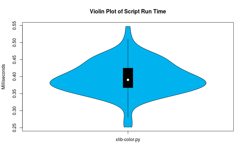
xlib-color.py
> xlib_color_py = dplyr::filter(run_time_comparison, script_name == "xlib-color.py") |
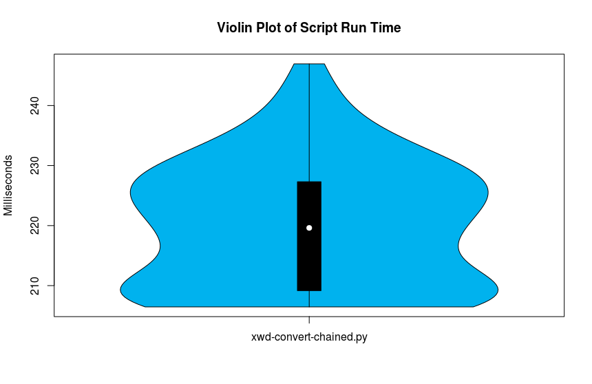
xwd-convert-chained.py
> xwd_convert_chained_py = dplyr::filter(run_time_comparison, script_name == "xwd-convert-chained.py") |
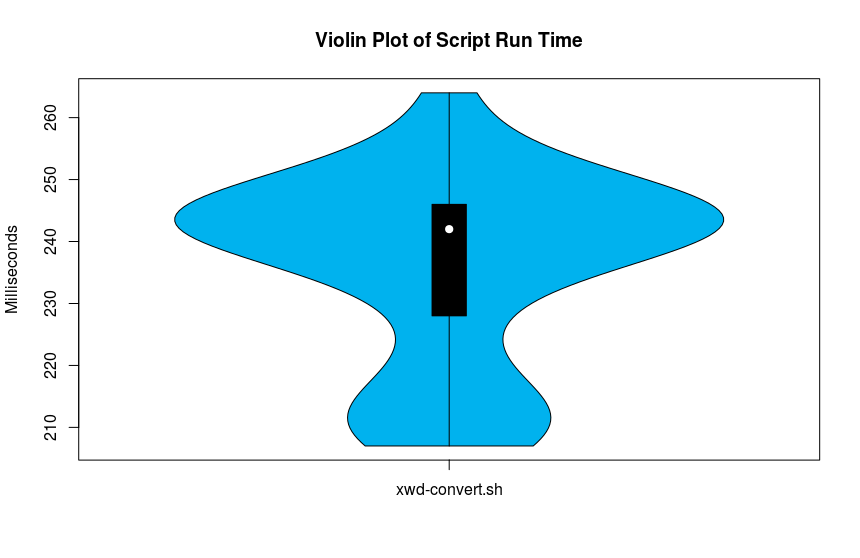
xwd-convert.sh
> xwd_convert_sh = dplyr::filter(run_time_comparison, script_name == "xwd-convert.sh") |
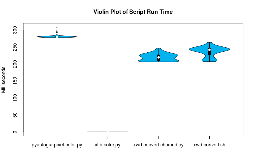
All Together
Because of xlib-color.py, this graph isn't terribly useful. There's too much range.
> png( |
Slow Only
This is one is a bit better. Unfortunately, it does a good job of highlighting how slow pyautogui can be.
> png( |
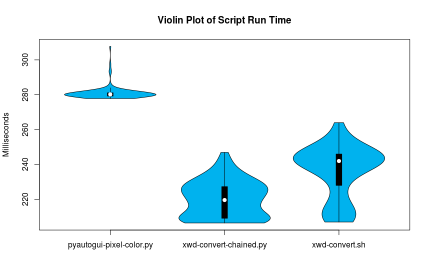
Conclusions
python-xlibis scary fast. That's so awesome.pyautoguiis slower than I thought. It does seem to maintain a fairly stable slow, pace, though, in comparison to the others.- Chaining commands via Python is actually, on average, faster than running things through
bash. I don't know if that's because of the additionalawkprocessing on the tail end ofxwd-convert.shor something else. It bears some investigation.